Training Area
Learn like us at the Neonatal Health Systems Lab
Epidemiology
The study of diseases at a population-level
In epidemiology we apply statistical and descriptive tools and techniques to assess disease trends in populations. Epidemiology research can have many implications at different levels of healthcare and health research. In our lab we apply epidemiology to assess associations (a statistical cause-effect relationship) between our exposures (variables which may be the cause for an effect of interest), such as organizational factors, and our outcomes (effect of interest).
There is a cautionary tale in statistics: correlation does not equal causation. Simply put, an exposure may seem to predict an outcome because as one occurs so does the other (for example, seeing more people carrying umbrellas and then it begins raining in the next few hours. If correlation was all that mattered, people carrying their umbrellas would be assumed to predict rain). However, that does not mean that the exposure actually causes the outcome (back to our example, people may have checked their weather app in advance and the rain was destined to happen before they grabbed their umbrellas). Similarly, in statistics and data modelling a statistical association does not necessarily mean that a true causal association exists between an exposure and outcome. For this reason epidemiologists turn to tools like the Directed Acyclic Graph (DAG) to logically justify causal relationships. These DAGs can be as simple as

Or as complicated as
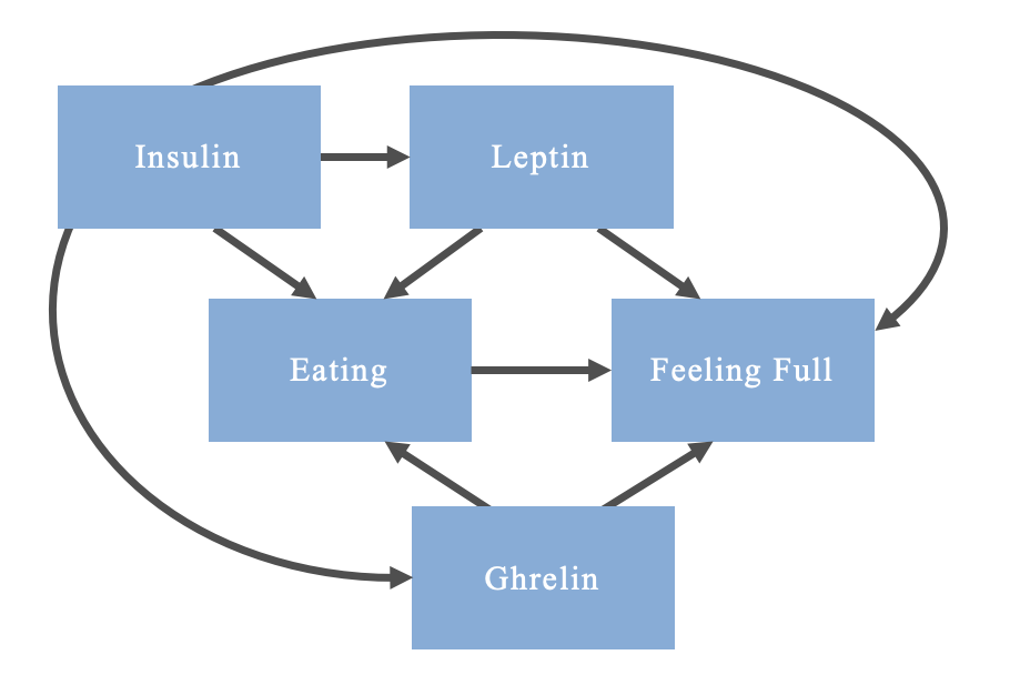
Note that this is an oversimplification of the relationship and mechanisms; some mechanisms are bidirectional, but DAGs are only able to account for unidirectional relations between a cause and effect (i.e., acyclic)
In creating these DAGs we are able to identify confounders. Confounders are variables which are a cause of both the exposure and the outcome in an association that is being assessed (e.g. leptin in the above DAG). These variables must be controlled for in the design or analysis stage of the study. If they are left uncontrolled, you risk biasing the association under assessment, potentially making a statistical association appear to exist when there is truly no causal relationship between a given exposure and an outcome.
For example, imagine you are creating a study comparing eating behaviours and satiety among body builders with non-body builders. If you notice that the body builders eat more and feel more hungry, you may incorrectly conclude that eating increases hunger. What you have failed to account for (among other things) is that leptin stimulates satiety. Leptin is a hormone produced by adipose tissue; presumably, unless participants struggle with leptin dysregulation, the body builders will have a lower body fat percentage than non-body builders, resulting in them feeling less satiated. Therefore, leptin confounds your relationship and needs to be accounted for in order to properly conclude that eating leads to feeling full.

There are certain principles that have helped to shape our understanding of confounding in epidemiology. One of these is Bradford Hill’s Criteria for causation, which has been adapted by Fedak et al. (2015) to account for its limitations in the 21st century. Principles and theoretical frameworks in epidemiology research are important to your study. Establishing a theoretical framework for a research question first requires building the body of evidence pertaining to the association being investigated.
Study Designs
The initial studies used to generate a research question in epidemiology are often referred to as Descriptive Studies. Descriptive studies are as the name implies—descriptive in nature. They are not conducted with the intent of rigorous analyses for a causal conclusion. In fact, these studies cannot establish causality, and should not be used with that intention. Instead, they are “hypothesis-generating”.
Among the most simplistic designs is a case report. Case reports are files which document a case for a person who experienced a particular outcome, often written by medical personnel. These reports may list contextual factors and biological data, but the risk factors provided should be interpreted with a grain of salt. A report could have documented someone who presented with nausea and an elevated blood pressure, which may have suggested that their elevated blood pressure contributed to the nausea (or vice versa). However, the nausea (along with the elevated blood pressure) could have been the result of a separate cause, such as anxiety from a stressful event. Or, the symptoms of anxiety may present as such in one person but not in three other people who go to an Emergency Room due to symptoms resulting from their anxiety. For these reasons, a singular case report can be insufficient to draw conclusions. You are not able to statistically assess for associations with a sample size of one.
Subsequently, following presentations of multiple patients with similar outcomes, a case series may be generated to document the outcome and to identify trends. These case series are simply a collection of case reports, with descriptives of commonalities to aid in further hypothesis generation. They are however limited in how they can be interpreted. A common trend may be alluring to draw conclusions regarding causes of a disease, but there is still a lack of statistical evidence. Additionally, when all you have are cases, you may feel inclined to assume correlations are causations. Returning to our example with anxiety, imagine that the case series reveal that many people who show up in the ER with anxiety are students at the affiliated college. You may feel inclined to conclude that students at that college may have higher anxiety rates than other people (which may be true), but without having assessed anxiety levels among other students in the area, or rates of anxiety at other hospitals, you may draw inaccurate conclusions. This is why non-diseased or non-exposed people are included in epidemiological studies: they act as a comparator group to statistically assess if a characteristic is more common among those with an outcome relative to those without the outcome.
A cross-sectional study provides more insight into the relationship, allowing you to include populations without an outcome or populations who were in a different exposure group. These studies are called “cross-sectional” because they capture a snapshot of the population at a point in time. This allows you to assess for correlations between variables and the outcomes between the comparator groups; these correlations can be analyzed using descriptive statistics to draw inferences and refine hypotheses. Cross-sectional studies can also be very useful to determine the prevalence of an outcome in a population. Still, further investigation will be required using Analytical Studies.
Analytical studies can be divided into experimental and observational designs, and involve statistical analyses of associations. Experimental designs are intervention-based, such as a Randomized Controlled Trial (RCT). RCTs are used in drug development, where people are divided into a group who receives the drug (exposed) and a group who does not (unexposed). Participants are then followed-up to assess for the outcome. In fact, follow-up is a critical element of analytical study designs. Follow-up ensures that there is a temporal relationship between exposures and outcomes, which is important for establishing causality: causes must precede effects.
Observational designs are popular in epidemiology. An observational design means that no intervention is applied by the researchers. This technique is particularly useful when exposing people to an intervention is not ethical, such as when studying environmental toxicity. Cohort studies are designed such that a cohort of people is followed through time to assess for whether or not an exposure of interest is associated with the outcome. These cohorts can be identified through different mechanisms, depending on the available data. A less resource-intensive approach is to select a cohort, determine who has the outcome, and then identify whether or not they were exposed prior to developing the outcome. This design is called a retrospective cohort study. In a prospective cohort study the cohort without the outcome is identified at the beginning of the study and then they are followed through time to determine if they develop the outcome. The exposure status is ascertained at the beginning.


An alternative design is a case-control study. This design is useful when a rare outcome is being assessed. In a case-control study, cases are identified as they develop the outcome and then controls are selected from the same population that the cases came from. Controls must be individuals without the outcome of interest. Subsequently, exposure status is ascertained for both the cases and controls in order to conduct the statistical analysis. Up to 4 controls may be selected per case included in the study.
All of these designs are valuable in describing the effects of exposures on outcomes, and can be measured using different measures of effects.
Measures of Disease Frequency and Effects
Measures of effects describe the association between exposures and outcomes in different studies. Measures of disease frequency describe the occurrence of a disease in a population.
Prevalence is the proportion of the cases in the population; obtained from cross-sectional studies
Incidence Rate is the rate which new cases occur; obtained from cohort studies
Incidence Proportion (i.e., Risk, Cumulative Incidence) is the average probability of an outcome occurring; obtained from cohort studies & RCTs
Odds is an estimation of risk; obtained from case-control studies
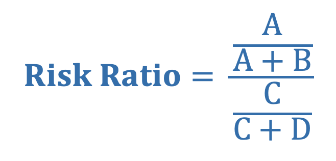
Risk Ratio (i.e., Relative Risk) is the ratio of the average risk of the outcome between the exposed and unexposed group
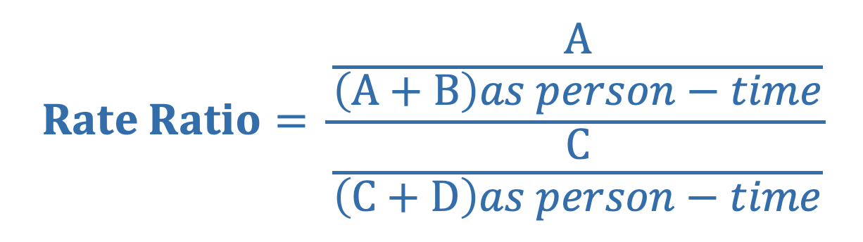
Rate Ratio is the ratio of the average rate of the outcome between the exposed and unexposed group (denominator is often person-time)
Odds Ratio is the ratio of the odds of exposure among those with the outcome, relative to the odds of exposure among those without the outcome
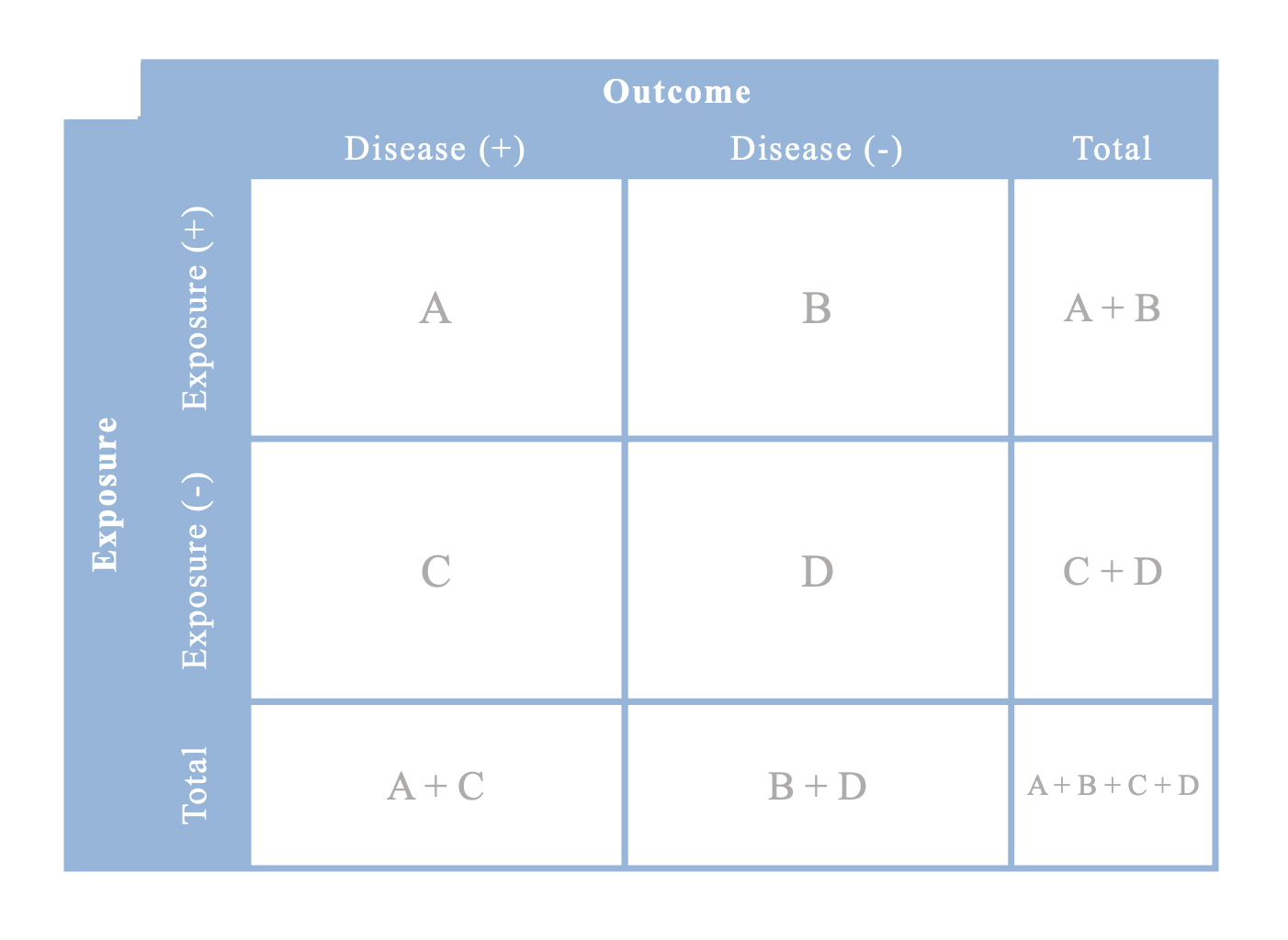
Contingency table for risk ratios or rate ratios
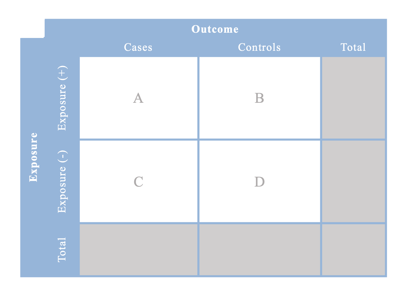
Contingency table for odds ratios

Note that you cannot calculate any totals in case-control studies because you hand-selected only a sample of cases and controls; the true enumeration of those who are exposed/unexposed and cases/controls in the cohort has not been completed
Economic Evaluations
The practice of comparing costs and outcomes between 2+ interventions
Economic evaluations are an important element of intervention-based research. Using economic evaluations enables decision-makers to determine which interventions best meet their needs and they are willing to invest in. The Canadian Agency for Drugs and Technologies in Health (CADTH) has developed guidelines to aid in the understanding and implementation of economic evaluation for health technologies in Canada.
There are multiple types of economic evaluations to represent the various measures of outcomes in cost analyses. A cost-effectiveness analysis (CEA) provides insight in the cost per unit measure of natural outcomes (e.g. cost per life saved). This analysis is often pursued in the form of a cost-utility analysis (CUA), where the measure of effectiveness is a measure of health status, such as a Quality-Adjusted Life Year (QALY). A QALY is a numerical representation of the effect of a health condition on someone’s quality of life. A cost-benefit analysis (CBA) is a similar idea, however the outcome is converted to a dollar value.
Economic Theories for Health Economic Evaluations
Economic evaluations are approached with the inspiration of economic theories. Utilitarianism is a prominent philosophy and perspective that deems that an action which does the most good for the most people, while minimizing harm, is the best course of action. As such, utility is a positive outcome resulting from an action. Welfarism is used as an economic theory that applies principles of utilitarianism, in which people are assumed to know what is best for their own welfare/well-being (i.e., utility). In welfarism, the intention is to improve the well-being of individuals without sacrificing the well-being of others.
Another economic theory in economic evaluations is the Capability Approach. This theory is rooted in a belief that improving people’s capabilities, which may occur by improving their functionings (ability to function), should be at the core of assessing health technologies. Whereas welfarism values the state of wellbeing or happiness, the capability approach values interventions to improve what someone could or would be able to do. In that sense, it is centred on improving opportunities for people.
Extra-Welfarism draws inspiration from both welfarism and the capability approach. Under extra-welfarist assumptions, the definition for utility includes “non-good characteristics such as health states and freedom of choice”. Thus, it expands the welfarist framework, but also tends to apply population-level assumptions about what an individual may define as good for their own well-being (e.g. health states are evaluated using population-based data).
When conducting an economic evaluation it is important to consider the economic theory behind the research as it contributes to the selection and defining of costs and outcomes in the study.
Elements in this passage on Welfarism, the Capability Approach, and Extra-Welfarism were adapted from a 2008 article by Coast, Smith, and Lorgelly (article).
Cost Perspectives
It is important when conducting an economic evaluation that the cost perspective is stated in the report. Stating a cost perspective is a fundamental way in which a researcher justifies why they included certain sources of costs when defining the costs in their evaluation. Three main perspectives include: a Ministry of Health Perspective, a Government Perspective, and a Societal Perspective.
In a Ministry of Health Perspective, the only costs included in the analysis are government expenditures on health and social care as a result of the intervention. These costs are combined with other government-borne costs (e.g. social assistance and disability payments) and tax revenues in a Government Perspective. Lastly, a Societal Perspective combines elements of both the Ministry of Health and Government perspectives, though it excludes sources such as tax revenues and disability payments, as they are treated as “transfer payments” and are not lost from the system being analyzed. Therefore, the societal perspective includes government-borne health, social care, and other costs, as well as health and social care expenditures covered by individuals or private insurance. Personal income and time are also included in these costs, and may be considered to reflect lost income, especially if time is taken off of work to participate in the intervention. Different cost perspectives can yield dramatically different cost estimates in economic evaluations. It is best practice to be transparent about costing when writing a report on an economic evaluation.
There are other elements of costing which can be useful to consider in economic evaluations, such as an opportunity cost. Opportunity costs are costs incurred by the loss or gain of potential revenue or assets. An example of an opportunity cost could be the travel time and lost wages of someone who has to travel from a rural community to an urban centre to attend a doctor’s appointment as a part of a study. These costs can be highly theoretical, but still valuable when weighing the costs and benefits of an intervention.
Thus, how we decide to measure costs and outcomes is important.

Costs and Outcomes
One principle that is highly recommended for economic evaluations is to apply a discounting rate of 3% (some may use 1.5% or 5%) to discount both costs and benefits in the evaluation as time progresses. Conceptually, discounting is used because it is believed that: people value money and health outcomes less in the future than in the present; there are opportunity costs associated with receiving benefits earlier; and uncertainty about the future needs to be accounted for by decreasing values. Both outcomes and costs need to be discounted to balance their values and not bias their weight in people’s decisions.
Health outcomes can be measured in a variety of ways. In many analyses it is common to see a Quality Adjusted Life Year (QALY) or a Disability Adjusted Life Year (DALY) used to describe the measure of benefit. A QALY is a measure of how a condition may alter one’s quality of life during the span of a year, essentially reducing that year lived to a fraction of a year. Conversely, a DALY estimates the number of years lost to a condition by accounting for both reductions in lifespan and reductions in quality of life due to a disability. Other measures of health outcomes and quality of life also exist. These measures of health outcomes are often obtained from study data with standardized instruments which gather people’s preferences and perceptions of a given condition.
There are standardized instruments for establish health-state preferences, allowing for comparisons of health between outcomes. A visual analogue scale is the simplest instrument. Participants can use a sliding scale to indicate how they think a health condition compares to perfect health. Standard gamble is an instrument involving repeated questions which compares people’s preferences between two health states, while incorporating probabilities in the decision-making process. Time trade-off operates in a similar manner, however, instead of selecting the health states based on probabilities, they indicate which health state they would rather experience, while considering how long they would be expected to live with each health state. Each of these instruments are better suited for certain applications, with their own respective strengths and limitations.
The Evaluation
The measure of evaluation for these analyses is often an Incremental Cost-Effectiveness Ratio (ICER). An ICER is an incremental increase in the ratio of costs to benefits for a given intervention. Comparing two ratios for two separate interventions allows you to compare which intervention is more cost-effective.
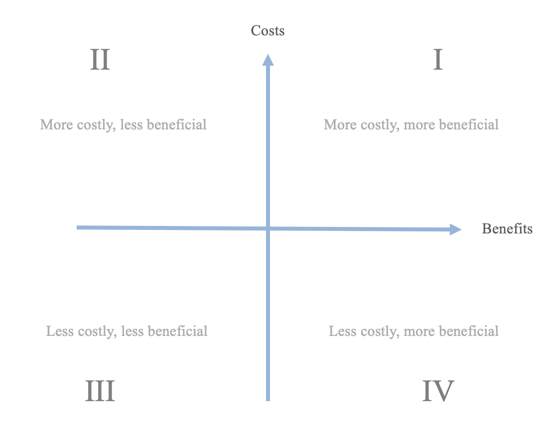
If the ICER of one intervention was placed at the origin of this plane, another intervention is more cost-effective if it lies in quadrant IV. In the case that the second intervention were to be in quadrant II, it would be clearly less cost-effective: anything in quadrants I and III would be unclear if they are better interventions.
Additional considerations may be involved if the evaluation employs a Willingness to Pay threshold. The willingness to pay threshold defines a ratio of costs relative to benefits that a decision-maker is willing to pay for an intervention. ICERs of interventions which fall below the threshold are eligible to be pursued.
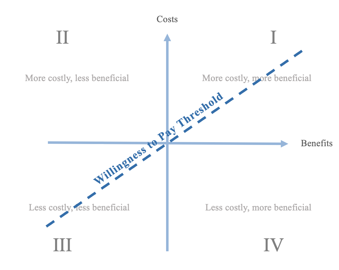
A similar threshold known as a Willingness to Accept threshold may be used when the intervention is being assessed under a different perspective. If a party is going to be involved in an intervention, they may be asked how much money they would be willing to accept per every unit of benefit (e.g., the government paying family members to care for an elderly member by themselves).
Modelling
Modelling for economic evaluations can be done in a number of ways. You can coincide a model of the probabilities of diseases and outcomes with the anticipated costs in order to generate an ICER for an economic evaluation. One example of a modelling technique is the decision analytic model, which can be used to generate a decision analytic tree. A decision analytic tree is an algorithm which assigns probabilities to outcomes, which are placed on different branches of the tree to represent the different paths which an event could follow. Each node (or “chance node”) in the tree represents a branching point, and all of the branches connected to the node should have probabilities which sum to 100%. The associated costs and benefits (e.g. QALY) for each outcome are assigned to the outcome, and are used to calculate estimated ICERs along the decision analytic tree.

Dynamic compartmental models are employed in both economic evaluations and infectious disease modelling. These models follow populations as they transition through diseased states, or compartments. There are variations of the models which can capture different disease trends (e.g., SIR, SIS, SEIR). S stands for Susceptible, and refers to someone who is susceptible of an infection. I is Infectious and refers to someone currently ill and able to infect others with their infection. R is Recovered, and is used to compartmentalize people who become immune or die as a result of the infection. Some models may be more complex; an SIS model (Susceptible-Infectious-Susceptible) may be used when people who became ill are able to be reinfected (e.g. after recovering from a bacterial infection). An SEIR (E represents Exposed) is used to model infections when there is an idea on how exposure contributes to the infection timeline and risks. Economic evaluations can accompany these models, and the models themselves can even be employed when conducting other modelling, such as the Markov model.
Markov models are a modelling technique which accounts for time-oriented events in the model. The model is comprised of Markov states (states which a person can be in within the model; similar to compartments), transition state probabilities (similar to the probabilities in a decision model), and cycles (i.e., discrete time periods). Costs and QALYs can be assigned to the different Markov states, and after running a cohort-based stimulation, a cost-effectiveness ratio can be determined at the end of the sequence.
There is flexibility in modelling economic evaluations. Each model comes with its own strengths and weaknesses; the decision when selecting a model comes down to what model best answers your question.
CHEERS
Economic evaluations should be conducted and reported under the guidance of the Consolidated Health Economic Evaluation Reporting Standards (CHEERS). This checklist promotes reporting consistency in economic evaluations. Time horizon, discount rate, and uncertainty are a few of the elements that the CHEERS guidelines advise for reporting.
Diagnostic-Related Groups
Grouping system for patients of similar case-mixes
Diagnostic-Related Groups (DRGs) were developed in the United States as a means to group patients by their “case-mix” for administrative purposes in assessing resource use. These case-mixes of patients may be similar based on their medical diagnosis, surgical procedures, age, or comorbidities, and thus require similar levels of intensity of care. Resource utilization patterns are important for healthcare management when evaluating and planning the distribution of resources based on predicted needs. Multiple iterations of the DRG have been created, with further development to include patient populations such as neonates.
Brief History of DRGs
Development of DRGs began in the 1960s at Yale University. The system was first used in the state of New Jersey for payment and reimbursement of healthcare facilities. Initial versions of DRGs typically encompassed a single organ system/medical specialty, which was further refined by a medical/surgical specification, often relying on hierarchies of the most significant diagnosis/procedure. In 1983, the DRG system was revised with the establishment of Medicare. Annual revisions have since been made by the Centers for Medicare and Medicaid Services, which has focused on updating DRGs for elderly populations and neglected neonate/pediatric populations. In 1987, New York State instituted a DRG system for non-Medicare patients that expanded the DRG system into All Patient DRGs (AP-DRGs). This system introduced pediatric and neonatal DRGs, which accounted for infant birthweight and CPAP/mechanical ventilation use, resulting in 34 neonatal AP-DRGs. All Patient-Related DRGs (APR-DRGs) were eventually developed with a severity of illness subclass and risk of mortality subclass to meet applications of the DRG system beyond healthcare costing/resource utilization.
Canada developed their own case-mix groups (CMGs) starting in 1983 by the Hospital Medical Records Institute, which was later transferred to the Canadian Institute of Health Information (CIHI). Since the 1980s, DRGs for neonates have been found to limited in their predictive abilities for resource utilization. Phibbs et al. (1986) evaluated the DRG system and found it to lack predictive power for length of stay and cost in Level-III NICUs. They also found that cost was most closely associated with birthweight and mechanical ventilation, followed by death, surgery, discharge and multiple birth.
This section was adapted from All Patient Refined Diagnosis Related Groups (APR-DRGs)—Methodology Review (2003), 3M Health Information Services.
Modern Case-Mix Groupings
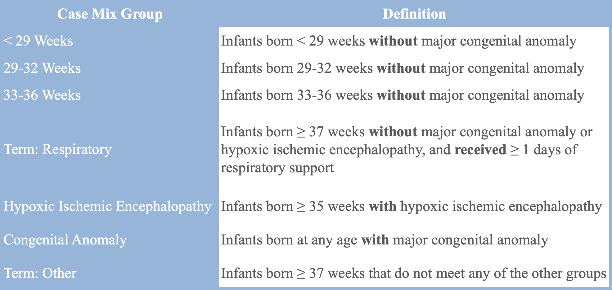
Most provinces in Canada use a tool equivalent to the DRG developed by CIHI known as Case-Mix Groups+ (CMG+) which primarily uses ICD-10 codes to group patients. In neonatal care, other case-mix groupings are also used: for example, Quebec uses the All Patient Related-DRG (APR-DRG). The Canadian Neonatal Network (CNN), a national organization affiliated with all tertiary-level Neonatal Intensive Care Units (NICUs) in the country, uses a unique set of case-mix groups. Their mutually exclusive groups are divided into infants <29 weeks gestational age, 29-32 weeks gestational age, 33-36 weeks gestational age, term infants on respiratory support, term infants with hypoxic ischemic encephalopathy, infants with a congenital anomaly, and term infants with other conditions.